Vector Indexes

Build and optimize LanceDB vector indexes, including IVF, HNSW and binary quantized indexes.

You can create and manage multiple vector indexes on any Lance dataset. LanceDB offers two vector indexing algorithms: Inverted File (IVF) and Hierarchical Navigable Small World (HNSW).

IVF + HNSW

In LanceDB, HNSW is not exposed as a top-level vector index. Instead, it’s available as a sub-index inside IVF partitions. What this means in practice is that vectors are first partitioned by IVF, then each selected partition is searched using an HNSW graph. LanceDB supports the unquantized variant IVF_HNSW_FLAT, along with quantized variants such as IVF_HNSW_PQ and IVF_HNSW_SQ. This combines IVF’s scalability with HNSW’s higher-recall ANN search within partitions.

Use this table to choose the right index and quantization type for your use case:

If your top priority is…	Use this index	Why	Typical compressed size vs. raw vectors
Highest recall / no quantization	IVF_HNSW_FLAT	Uses raw vectors inside the IVF+HNSW structure, avoiding quantization loss.	Around raw vector size plus HNSW graph overhead
Best recall/latency trade-off	IVF_HNSW_SQ	Combines IVF partitioning with HNSW graph search for strong quality at low latency.	Typically a little larger than 1/4 of raw size
Maximum compression	IVF_RQ	RaBitQ-style quantization with very strong compression.	Around 1/32 of raw size
Higher accuracy at small dimensions (dimension <= 256)	IVF_PQ	On small-dimensional vectors, IVF_PQ often provides higher accuracy with similar performance compared to IVF_RQ.	Usually 1/64 to 1/16 of raw size (depends on num_sub_vectors)

If your vector search frequently includes metadata filters (where(...)), prefer IVF_RQ or IVF_PQ. In filtered workloads, HNSW-backed IVF indexes such as IVF_HNSW_FLAT and IVF_HNSW_SQ can show higher latency variance.

Compression ratios are practical rules of thumb and can vary with vector distribution, metric, and configuration. For small dimensions, choose IVF_PQ for accuracy, not for guaranteed higher compression than IVF_RQ.

Index Tuning

Start with these values, then tune for your workload:

• HNSW-backed IVF indexes (IVF_HNSW_FLAT, IVF_HNSW_SQ, IVF_HNSW_PQ)
  • num_partitions: start at num_rows // 1,048,576 (rounded to an integer)
  • Lower num_partitions can reduce search latency, but index build may become slower because partitions are larger.
  • ef_construction: start at 150; increase for better recall, decrease for faster indexing.
• IVF_RQ
  • num_partitions: start at num_rows // 4096 (rounded to an integer). This is a strong default for most datasets.
• IVF_PQ
  • num_partitions: start at num_rows // 4096 (rounded to an integer).
  • num_sub_vectors: start at dimension // 8. Increase for better recall, decrease for faster search and smaller indexes.
  • For small dimensions (dimension <= 256), IVF_PQ is often preferred over IVF_RQ for better accuracy at similar query performance.

Operational checks

For vector indexes, make sure to use the same distance metric when creating and querying the index. After appends or other writes, use optimize() to fold new rows into existing indexes, then check index_stats(...) or wait_for_index(...) to confirm that the index has caught up. wait_for_index(...) waits until the named indexes exist and report num_unindexed_rows == 0, and can time out if writes keep adding unindexed rows.

Unless specified otherwise, vector indexing defaults to IVF_PQ, and scalar index creation defaults to BTree. BTree and Bitmap indexes target scalar columns, not list columns; use LabelList for list containment filters.

Understanding Vector Indexes

An ANN (Approximate Nearest Neighbors) index is a data structure that quickly produces an approximate solution to the $k$-Nearest Neighbors (kNN) problem. It greatly improves upon the runtime of a brute-force kNN search, while admitting a slight decrease in accuracy. LanceDB uses the disk-based indexing technique IVF-PQ, discussed below.

LanceDB differs from other vector databases in that it is built on top of Lance, an open-source columnar data format designed for performant ML workloads and fast random access. Due to the design of Lance, LanceDB’s indexing philosophy adopts a primarily disk-based indexing philosophy.

Inverted File Index (IVF) and IVF-PQ

LanceDB uses IVF-PQ indexing, which combines the clustering-based Inverted File Index (IVF) with Product Quantization (PQ) to efficiently compress embeddings. We primarily discuss the IVF indexing technique here.

An IVF index facilitates rapid nearest neighbor searches by drastically reducing the search space.

Given a large set of stored vectors, the algorithm to produce an IVF index first computes a set of centroids corresponding to an approximate solution to the $k$-means clustering problem. The centroids are then used to partition the set of vectors as follows: each vector is assigned to the centroid nearest to it in the $\ell_2$ (or user-specified) metric. The set of vectors assigned to a centroid is called its cluster. This data is then recorded as an index which identifies each centroid with its cluster.

The following image shows a $2$-dimensional Euclidean space partitioned according to this algorithm. The colored marks denote centroids.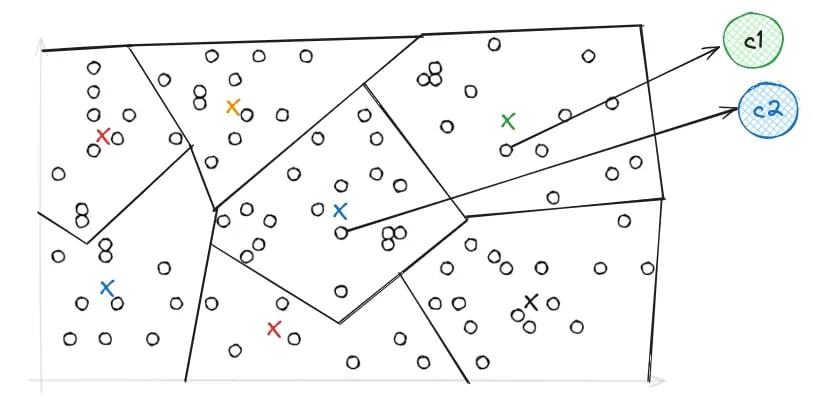

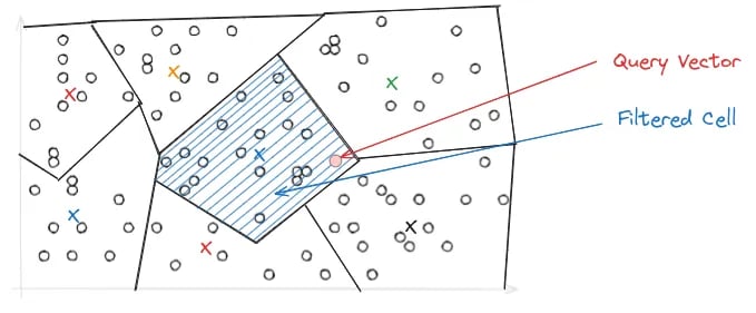
To process a nearest neighbors query, instead of a brute-force comparison of the queried vector to every stored vector, the system can instead search the much-smaller set of *centroids$ for a closest match, then execute a brute-force comparison against its associated cluster. This technique quickly eliminates the vast majority of clusters from the search space. Furthermore, since each centroid is relatively close to points in its cluster, we are likely to produce an approximately correct result.

here vv During query time, depending on where the query lands in vector space, it may be close to the border of multiple Voronoi cells, which could make the top-k results ambiguous and span across multiple cells. To address this, the IVF-PQ introduces the nprobe parameter, which controls the number of Voronoi cells to search during a query. The higher the nprobe, the more accurate the results, but the slower the query.

Hierarchical Navigable Small World (HNSW)

Approximate Nearest Neighbor (ANN) search is a method for finding data points near a given point in a dataset, though not always the exact nearest one. HNSW is one of the most accurate and fastest Approximate Nearest Neighbour search algorithms, It’s beneficial in high-dimensional spaces where finding the same nearest neighbor would be too slow and costly.

Types of ANN Search Algorithms

Approximate Nearest Neighbor (ANN) search is a method for finding data points near a given point in a dataset, though not always the exact nearest one. For example, HNSW is an ANN index that performs well in high-dimensional spaces where other techniques prove too slow and costly.

There are three main types of ANN search algorithms:

• Tree-based search algorithms: Use a tree structure to organize and store data points.
• Hash-based search algorithms: Use a specialized geometric hash table to store and manage data points. These algorithms typically focus on theoretical guarantees, and don’t usually perform as well as the other approaches in practice.
• Graph-based search algorithms: Use a graph structure to store data points, which can be a bit complex.

HNSW is a graph-based algorithm. All graph-based search algorithms rely on the idea of a $k$-nearest neighbor (or $k$-approximate nearest neighbor) graph, which we outline below.
HNSW also combines this with the ideas behind a classic 1-dimensional search data structure: the skip list.

Understanding $k$-Nearest Neighbor Graphs

The $k$-nearest neighbor graph actually predates its use for ANN search. Its construction is quite simple:

• Each vector in the dataset is given an associated vertex.
• Each vertex has outgoing edges to its k nearest neighbors. That is, the k closest other vertices by Euclidean distance between the two corresponding vectors. This can be thought of as a “friend list” for the vertex.
• For some applications (including nearest-neighbor search), the incoming edges are also added.

Eventually, it was realized that the following greedy search method over such a graph typically results in good approximate nearest neighbors:

• Given a query vector, start at some fixed “entry point” vertex (e.g. the approximate center node).
• Look at that vertex’s neighbors. If any of them are closer to the query vector than the current vertex, then move to that vertex.
• Repeat until a local optimum is found.

The above algorithm also generalizes to e.g. top 10 approximate nearest neighbors.

Computing a $k$-nearest neighbor graph is actually quite slow, taking quadratic time in the dataset size. It was quickly realized that near-identical performance can be achieved using a k-approximate nearest neighbor graph. That is, instead of obtaining the $k$-nearest neighbors for each vertex, an approximate nearest neighbor search data structure is used to build much faster.
In fact, another data structure is not needed: This can be done “incrementally”. That is, if you start with a k-ANN graph for n-1 vertices, you can extend it to a k-ANN graph for n vertices as well by using the graph to obtain the k-ANN for the new vertex.

One downside of k-NN and k-ANN graphs alone is that one must typically build them with a large value of k to get decent results, resulting in a large index.

Hierarchical Navigable Small Worlds (HNSW)

HNSW builds on k-ANN in two main ways:

• Instead of getting the k-approximate nearest neighbors for a large value of k, it sparsifies the k-ANN graph using a carefully chosen “edge pruning” heuristic, allowing for the number of edges per vertex to be limited to a relatively small constant.
• The “entry point” vertex is chosen dynamically using a recursively constructed data structure on a subset of the data, similarly to a skip list.

This recursive structure can be thought of as separating into layers:

• At the bottom-most layer, a k-ANN graph on the whole dataset is present.
• At the second layer, a k-ANN graph on a fraction of the dataset (e.g. 10%) is present.
• At the Lth layer, a k-ANN graph is present. It is over a (constant) fraction (e.g. 10%) of the vectors/vertices present in the L-1th layer.

Then the greedy search routine operates as follows:

• At the top layer (using an arbitrary vertex as an entry point), use the greedy local search routine on the k-ANN graph to get an approximate nearest neighbor at that layer.
• Using the approximate nearest neighbor found in the previous layer as an entry point, find an approximate nearest neighbor in the next layer with the same method.
• Repeat until the bottom-most layer is reached. Then use the entry point to find multiple nearest neighbors (e.g. top 10).

Using Vector Indexes

Manual Indexing

If using LanceDB OSS, you will have to create the vector index manually, by calling table.create_index(), and updating the index as new data arrives and tuning its parameters is also a manual process.

Automatic Indexing

Enterprise-only Vector indexing is managed automatically in LanceDB Enterprise. When a table is created in LanceDB Enterprise, the system asynchronously updates and optimizes the index as a background process:

• Infers vector columns from the schema
• Optimizes the IVF_PQ index without manual configuration
• Automatically manages indexing parameters

The default distance is l2 (the Euclidean $\ell_2$ norm).

You can call create_index() with different parameters to create a new index — this replaces any existing index. Although the create_index API returns immediately, the building of the vector index is asynchronous. To wait until all data is fully indexed, you can specify the wait_timeout parameter.

Use the same distance metric for index creation and search. Once a vector index exists, queries use the metric stored with that index. If you need to confirm an async build or refresh is finished, wait_for_index(...) waits for the named index to exist and for index_stats(...) to report num_unindexed_rows == 0; it can time out if new writes keep arriving.

Rows appended after an index build remain outside that index until optimization refreshes it. Normal search still checks those unindexed rows with a slower fallback path; fast_search() skips that fallback and searches only indexed rows.

Example: Construct an IVF Index

In this example, we will create an index for a table containing 1536-dimensional vectors. The index will use IVF_PQ with L2 distance, which is well-suited for high-dimensional vector search.

Make sure you have enough data in your table (at least a few thousand rows) for effective index training.

Index Configuration

Sometimes you need to configure the index beyond default parameters:

• Index Types:
  • IVF_HNSW_FLAT: highest recall, with no vector quantization
  • IVF_HNSW_SQ: best recall/latency trade-off
  • IVF_RQ: best compression for large, high-dimensional datasets
  • IVF_PQ: often higher accuracy than IVF_RQ for small dimensions (<= 256) at similar query performance
• metrics: default is l2, other available are cosine or dot
  • When using cosine similarity, distances range from 0 (identical vectors) to 2 (maximally dissimilar)
• num_partitions: use index-specific starting points from the section above:
  • HNSW-backed IVF indexes (IVF_HNSW_FLAT, IVF_HNSW_SQ, IVF_HNSW_PQ): num_rows // 1,048,576
  • IVF_RQ and IVF_PQ: num_rows // 4096
• target_partition_size: alternative IVF sizing knob that asks LanceDB to derive the partition count from a target number of rows per partition. If you set both num_partitions and target_partition_size, num_partitions takes precedence.
• num_sub_vectors: applies to IVF_PQ; start with dimension // 8. Larger values often improve recall but can slow search.

Let’s take a look at a sample request for an IVF index:

1. Setup

Connect to LanceDB and open the table you want to index.

2. Construct an IVF Index

Create an IVF_PQ index with cosine similarity. Specify vector_column_name if you use multiple vector columns or non-default names. For a vector field nested inside a struct, use dot notation (e.g. image.embedding); see Selecting the vector column for the full syntax. You can switch index_type to IVF_RQ, IVF_HNSW_SQ, or IVF_HNSW_FLAT depending on your recall/latency/compression target.

Indexing nested vector fields

If your vector column lives inside a struct, pass its full dotted path as vector_column_name. The same path is used at query time and is what list_indices() reports under columns:

Nested paths follow Lance field-path semantics: dot-separate each struct field from root to leaf (for example, image.thumbnail.embedding). The same convention applies to FTS and scalar indexes.

Async API and Config Objects

With asynchronous Python connections, create vector indexes with await table.create_index("vector", config=...). The config object carries the same index choices you configure in the synchronous API, such as distance metric, partition count, and quantization settings:

Use these Python config classes for the index types shown on this page:

Index type	Python config class
IVF_FLAT	IvfFlat
IVF_PQ	IvfPq
IVF_RQ	IvfRq
IVF_SQ	IvfSq
IVF_HNSW_FLAT	IvfHnswFlat
IVF_HNSW_PQ	IvfHnswPq
IVF_HNSW_SQ	IvfHnswSq

3. Query the IVF Index

Search using a random 1,536-dimensional embedding.

Search Configuration

Core knobs available on a vector search call:

Parameter	Description
limit	Number of results to return (k).
nprobes	Shorthand that sets both minimum_nprobes and maximum_nprobes to the same value. LanceDB auto-tunes this by default.
minimum_nprobes	Partitions that are always scanned. Higher values raise recall at the cost of latency.
maximum_nprobes	Upper bound on partitions scanned. The partitions above minimum_nprobes are only searched if the initial pass does not return enough results — useful for narrow filters. Set to 0 to remove the cap.
ef	HNSW search-time exploration factor. Relevant for IVF_HNSW_FLAT and IVF_HNSW_SQ; start around 1.5 * k and increase up to 10 * k for higher recall.
refine_factor	Reads additional candidates and reranks them in memory to recover recall lost to quantization.

Filtered queries and adaptive nprobes. When a where(...) filter is active, LanceDB starts by scanning minimum_nprobes partitions and only extends toward maximum_nprobes if fewer than limit rows survive the filter. Setting minimum_nprobes == maximum_nprobes (or calling nprobes(n)) disables this adaptive behavior and fixes the partition count.

Recommended nprobes behavior by index type:

Index type	Guidance
IVF_HNSW_FLAT, IVF_HNSW_SQ	Keep the auto-tuned nprobes, then tune ef first. Expect higher latency variance under filtered search.
IVF_RQ	Keep auto-tuned nprobes; raise only when recall is insufficient.
IVF_PQ	Keep auto-tuned nprobes; raise when recall is insufficient. Often preferred over IVF_RQ when dimension <= 256.

Advanced Search Controls

These controls are useful for thresholded retrieval, recall measurement, and working around index-level metric constraints.

Method	Description
distance_range(lower_bound, upper_bound)	Return only rows whose distance falls within [lower_bound, upper_bound). Either bound is optional. Useful for near-duplicate detection or “close-enough” matching.
bypass_vector_index()	Skip the ANN index and perform an exhaustive (flat) scan. Primary uses: (1) compute ground-truth results to measure ANN recall@k, and (2) query with a metric the index was not built for (e.g., a non-cosine query on a multivector column).

Thresholding with distance_range:

Measuring recall with bypass_vector_index:

Compare ANN results against a flat-scan ground truth to compute recall@k. This is the standard way to pick nprobes for your workload.

Flat search is $O(n)$ — reserve bypass_vector_index() for sampled recall measurements or small tables, not production queries.

Multivector indexing currently requires distance_type="cosine" — l2 is rejected at index-creation time. That restriction is why bypass_vector_index() is the escape hatch for non-cosine queries on a multivector column: the metric you want at query time cannot be served by the index, so you fall back to a flat scan. See Multivector Search for the full rules.

Example: Construct an HNSW Index

Index Configuration

There are four key parameters to set when constructing an HNSW index:

• index_type: choose IVF_HNSW_SQ for a strong recall/latency/size trade-off, or IVF_HNSW_FLAT when you want the IVF+HNSW structure without vector quantization.
• metric: The default is l2 euclidean distance metric. Other available are dot and cosine.
• m: The number of neighbors to select for each vector in the HNSW graph.
• ef_construction: The number of candidates to evaluate during the construction of the HNSW graph.

1. Construct an HNSW Index

The snippet below uses IVF_HNSW_SQ. If you want the unquantized variant, change index_type to IVF_HNSW_FLAT.

2. Query the HNSW Index

Example: Construct a Binary Vector Index

Binary vectors are useful for hash-based retrieval, fingerprinting, or any scenario where data can be represented as bits.

Index Configuration

• Store binary vectors as fixed-size binary data (uint8 arrays, with 8 bits per byte). For storage, pack binary vectors into bytes to save space.
• Index Type: IVF_FLAT is used for indexing binary vectors
• metric: the hamming distance is used for similarity search
• The dimension of binary vectors must be a multiple of 8. For example, a 128-dimensional vector is stored as a uint8 array of size 16.

IVF_FLAT + hamming is the only supported path for binary vectors.

• hamming distance is only valid on packed binary (uint8) data; it is rejected on float vector columns.
• Quantized index types (IVF_PQ, IVF_RQ, IVF_SQ, IVF_HNSW_PQ, IVF_HNSW_SQ) do not accept binary inputs — their distance_type is restricted to l2, cosine, or dot.

1. Create Table and Schema

2. Generate and Add Data

3. Construct the Binary Index

4. Vector Search

Check Index Status

Vector index creation runs in the background and may take some time to complete. While it is ongoing, you can check its status either programmatically through the API or from the LanceDB Enterprise UI.

In the LanceDB Enterprise UI, navigate to your table page - the “Index” column reflects each column’s index status: it is blank when no index exists, shows an “in progress” label while the index is being built, and shows the index type once the build completes.

Programmatically, use list_indices() and index_stats(). By default, the index name is formed by appending _idx to the column name (e.g., a keywords_embeddings column produces keywords_embeddings_idx). Note that list_indices() only returns information after the index is fully built. To wait until all data is fully indexed, you can specify the wait_timeout parameter on create_index() or call wait_for_index() on the table.

Each entry returned by list_indices() also carries detailed per-index metadata, so you can inspect an index without a follow-up index_stats() call. Node.js exposes the same fields in camelCase (num_indexed_rows → numIndexedRows):

Field	What it tells you
num_indexed_rows, num_unindexed_rows	Index coverage over the table
size_bytes	Total size of the index files on disk
num_segments, index_version	On-disk layout and format version
created_at	Creation time (ms since the Unix epoch in Node.js)
index_uuid, type_url	Internal identifiers for the index segment
index_details	Type-specific details (e.g. IVF partition counts or quantization settings)

These fields are populated for local and embedded tables. On LanceDB Enterprise remote tables they are returned as None / undefined until the server response surfaces them.

Custom Index Names

The {column}_idx suffix is a default convention, not the only supported naming path. Pass name=... to create_index() to override it — useful when you want to manage multiple indexes on the same column (for example, side-by-side IVF_PQ and IVF_HNSW_SQ builds) or when you script index replacement by name. Once set, list_indices(), index_stats(name), and wait_for_index([name]) all reference the custom name.